One brick at
a time.
Marmon’s example kiln car held 28,800 bricks. In six days, our team built a tabletop prototype that could find a reachable brick, judge its colour, and tell a Franka arm where to pick it.
Follow one camera frameFrom kiln car to lab table
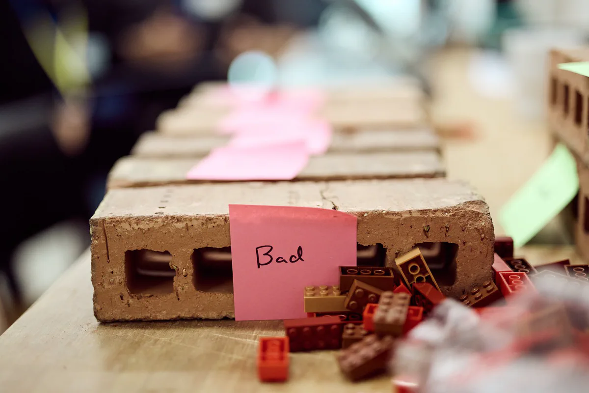
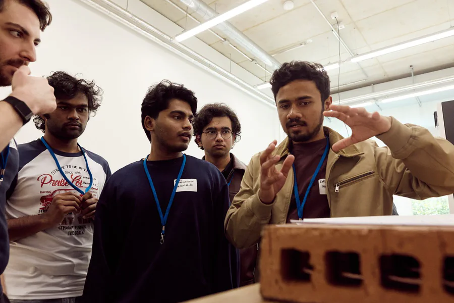
After firing, every brick on a kiln car has to be inspected, sorted by shade, and restacked onto pallets. Marmon challenged us to automate this unloading step, known as dehacking.
On our lab table, a woven stack of LEGO bricks stood in for a kiln car. The first decision was the same at either scale. Which brick can the robot pick without disturbing the stack?
My role on KalmanKrew
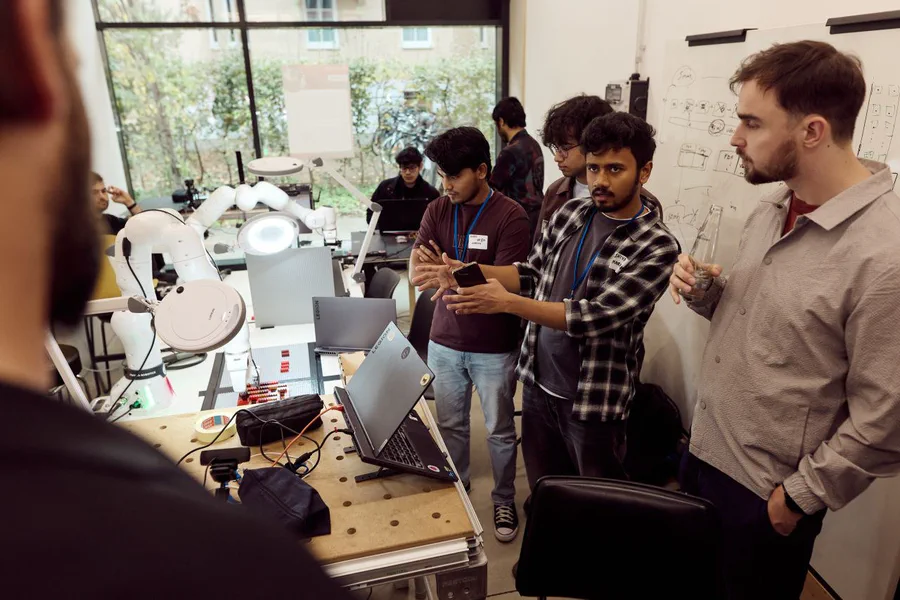
I led perception for the LEGO demo, taking the pipeline from raw camera frames to 3D targets for the motion planner.
- Perception: top-layer detection, size-based mask cleanup, colour classification and 3D pose export.
- Tooling: RGB-D capture, live detection and a modular runner for replaying recorded frames.
- On the robot: tuned grasps with the manipulation team and tested the full sorting loop.
From 61 masks to 22 pick targets
The camera sees the top layer, parts of lower layers, and loose bricks around the stack. Select a stage below to see how one RealSense frame becomes a set of 3D pick targets. You can also use the arrow keys after focusing a stage.
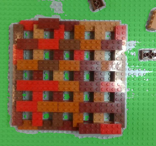 1 RGB-D frame
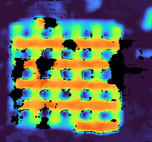 height map
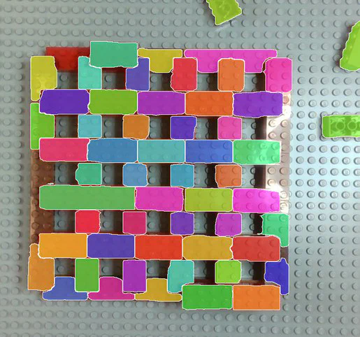 61 masks
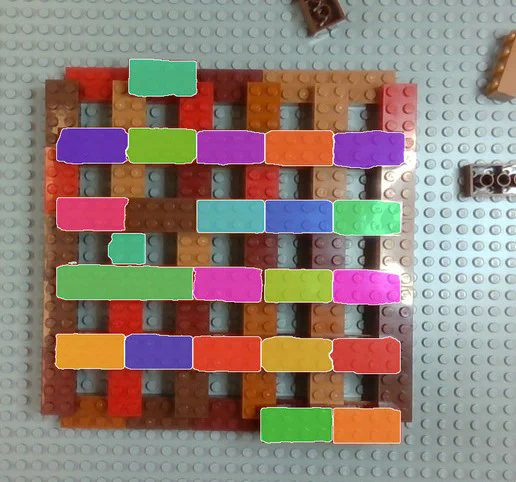 23 masks
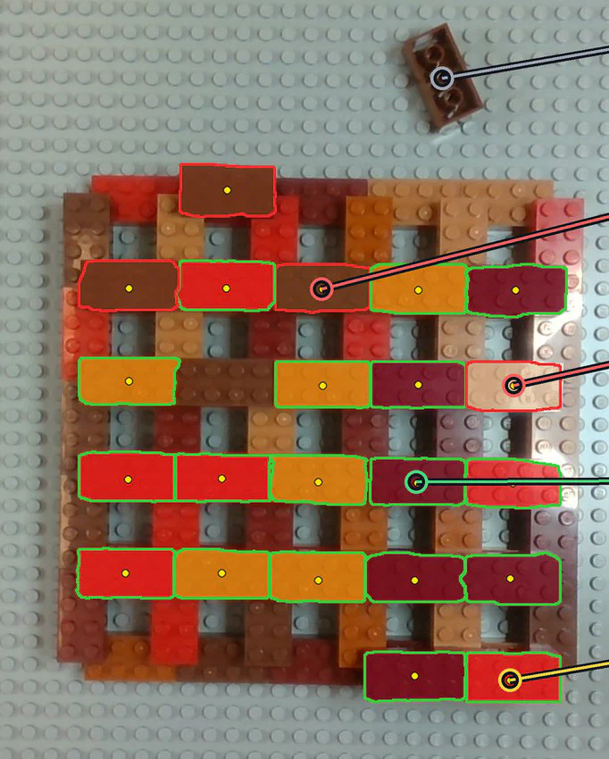 22 targets · 18 ✓ · 4 ✗
The wrist-mounted D435 captures an aligned colour + depth frame. RANSAC fits the dominant plane (green tint) — that is the table. Those same table pixels later serve as the white reference for colour.
Every depth pixel is back-projected and measured against the table plane. Warmer = higher, so the top layer of the stack stands out before any learning is involved.
A single text prompt returns instance masks for every visible brick — top layer, lower layers and loose ones alike. Colours here are just instance IDs.
A height histogram finds the highest substantial surface; only masks within one brick height (≈ 9.6 mm) of it survive. Lower layers and loose table bricks drop out.
A brick-size prior splits merged masks and rejects partial ones. Each brick is colour-classified in CIELAB and gets a fitted centre and yaw: green = accept, red = scrap, yellow dot = grasp centre.
One real capture from the RealSense D435, top-down over the LEGO stack. Stage images from the team's annotated pipeline figure.
Which bricks are reachable?
SAM 3 is very good at finding brick-shaped regions, but it has no notion of physical size. Two touching bricks can come back as one mask. A brick half-hidden under the layer above still looks like a brick, and so does the side face of an edge brick.
To fix this, I project each top-layer mask onto the table plane and measure its footprint in millimetres. I then compare that against a known brick size: L × W × H ≈ 30 × 15 × 10 mm. The prior then makes one of four calls:
≈ L × W
One clean brick
keepW × n·L
Bricks SAM merged
split into nW × < L
Mostly hidden by the layer above
reject< W wide
Side face of an edge brick
rejectEvery brick that survives gets a fitted L × W footprint. That gives its centre in the camera frame, its yaw on the table and its layer index, which is exactly what a grasp planner needs.
Which pile takes each brick?
The lab had bright desk lamps, glare on glossy plastic and shifting exposure. Matching raw RGB values would have mislabelled bricks constantly. The classifier corrects for that in three steps:
- White-balance on the table. The plane fit already says which pixels are table, so the colour model uses them as a grey reference in linear RGB.
- Measure the clean interior. Colour is sampled inside the fitted footprint, away from the edges. The darkest 15 % (shadows) and brightest 10 % (glare) are dropped.
- Match in CIELAB with a shared offset. One bounded Lab offset is fitted jointly across all bricks in the frame to absorb exposure drift. Then each brick takes its nearest reference colour, with a confidence from distance and margin.
Counts from the capture above.
Where should the gripper go?
Perception ends at a clean, documented contract. For every brick, the pipeline writes a 3D box in the camera optical frame (x right, y down, z forward, metres). The robotics side applies the hand-eye transform and plans the motion.
# per brick → bricks.json, poses.csv
id, colour, quality, confidence
layer           # index in the stack
centre_xyz      # box centre [m]
top_centre_xyz  # top face   [m]
yaw             # on the table
size_lwh        # fitted size
corners[8]      # top 0–3, bottom 4–7
I also wrapped the stages in a modular pipeline runner. It can capture a fresh frame or replay a recording, run segmentation, classification and pose export as separate processes, and give every run its own timestamped folder. If any stage fails, it stops and writes an explicit INCOMPLETE.json, so stale results are never silently reused.
Pick, place, look again
Even a successful pick can nudge the next brick out of position. The Franka picks a few bricks, returns to its observation pose, and rescans before committing to the next set of targets.
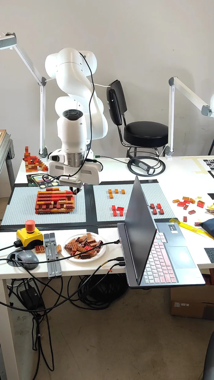
I helped tune and test the grasping side alongside our manipulation teammates. Most of the work went into details that only show up on real hardware:
- Grasp width and force for small, glossy 2×4 bricks
- Pre-grasp clearance and offsets so the fingers don't hit neighbouring bricks
- 3D-printed gripper fingers
- Varying layer heights as the stack shrinks
- A camera-to-gripper transform taken from CAD and refined on the robot
We demonstrated sorting on the Franka. Measuring pick success across repeated trials is the next step.
The final pitch
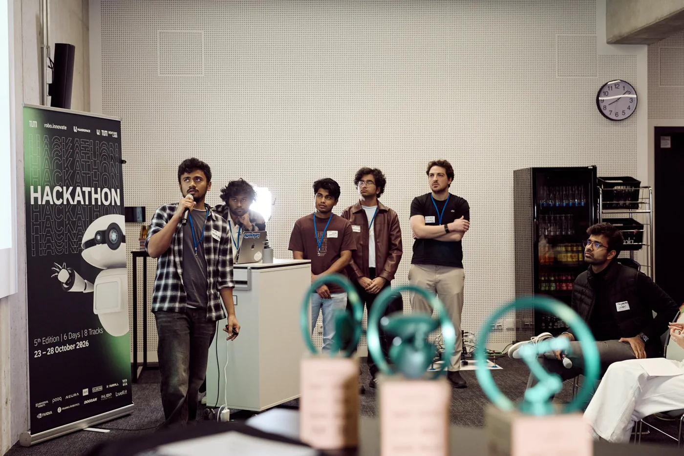
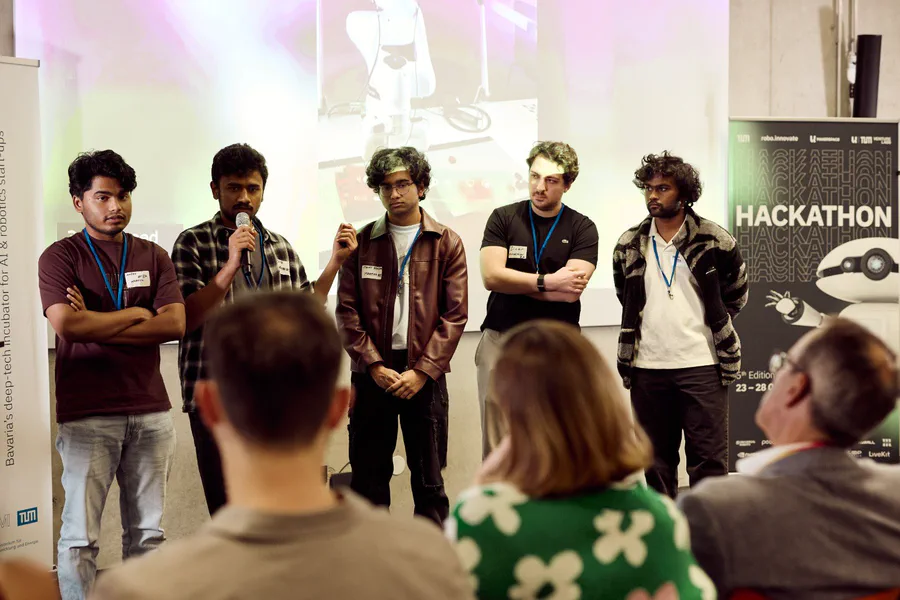
On day six, I presented three parts of the same idea to the jury. The Franka showed how to unload a stack, the real-brick inspector showed how to grade fired bricks, and the simulation showed how those steps could fit into a factory line.
Beyond the lab table
My teammates built two companion prototypes.
Grading real fired bricks
SAM 3 masks, hand-crafted colour and texture features, and DINOv2 patch features, fused through two linear SVMs. On 258 photos of the 10 sponsor samples, 9 of 10 bricks were graded correctly: all 4 good bricks accepted, 5 of 6 bad ones rejected.
Scaling the idea up
A simulated line covering dehacking, inspection, reject removal and palletizing, with a nominal throughput of ≈ 6,400 bricks per hour. The throughput estimate comes from scripted motion and simulated shade labels.
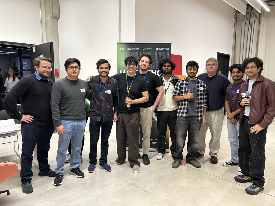
Six days in Munich
What I’d take into the next project
Use depth to narrow the search
A plane fit and a height histogram narrowed the candidate masks to the working layer. That made it easier to trace failed picks back to the geometry or the mask.
Use the world as a reference
The table doubled as a white reference, and one Lab offset per frame absorbed exposure drift. Both were more reliable than tuning camera settings for every lighting change.
Rescan beats predict
Rescanning after a few picks handled disturbed bricks and failed motions far better than trying to plan the whole stack from one frame.
Validate on unseen bricks
The inspector was evaluated on ten physical samples. Testing on unseen bricks and measuring pick success across repeated runs would show how well the system generalises.
Team KalmanKrew: Shiva Rudra (perception, pitch), Varun Teja (perception and real-brick classification), Tanay Ranjan (perception–manipulation integration, pick-and-rescan loop), Ameed Nazhurudeen (manipulation), and Ahmet Sinan Erdem (vision and simulation). Mentored by Peter So; challenge hosted by Jeff Garascia and Michael Ostrow from Marmon.

Shiva Rudra Lolla
Robotics Researcher
My research interests include autonomous systems and perception. Drop me a message if you want to connect!