A parallel four-bar mechanism is being used as a new type of wheel-legged robot, and two controllers are designed to ensure stable motion - the linear quadratic regulator (LQR) and fuzzy proportion differentiation (PD) jumping controller. The robot is equipped with the ability to jump over obstacles and navigate rough terrain. The height of the jump trajectory adjusts based on changes in the link angle of the parallel four-bar linkage mechanism, enhancing the robot’s ability to tackle vertical obstacles. The two modes of operation of the system:

• Self-balance: using LQR controller. To linearize the nonlinear state-space model about the equilibrium point(taking angular conditions as zero). Straight line motion(no steering can be assumed in the initial stage).
• Jumping: using a Fuzzy controller. To use Fuzzy conditions to switch between Stance and Flight stages and get the controller output accordingly. The kinematics of the robot are given as follows:

Self-Balance Mode

Mathematical Model for Self Balance Mode:

The robot’s balance and speed are regulated using the Linear Quadratic Regulator (LQR) technique. The equation for the state of the linear time-invariant system is: x_dot(t) = Ax(t) + Bu(t). The LQR controller works only on linear systems. But, our system is nonlinear with dynamics given as follows:

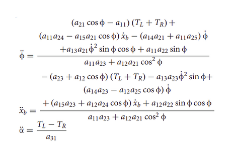
On converting it into matrix form by taking 6 states:

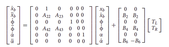
where:

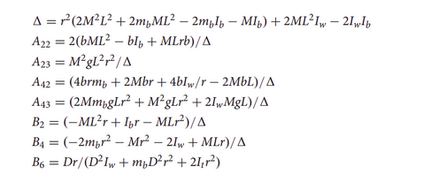
Here,

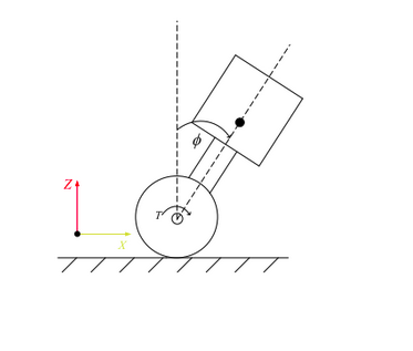
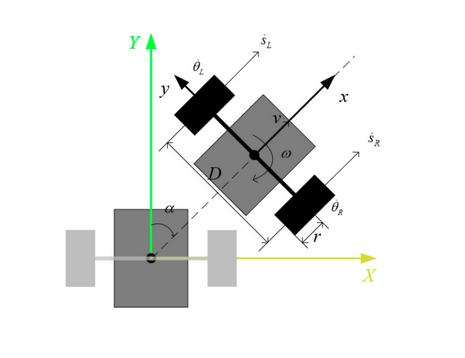
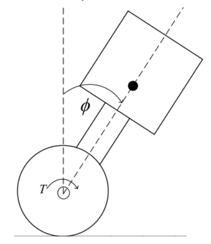
• xb is the forward displacement of the point of contact with the ground
• alpha is the steering angle
• phi is the tilt angle of the robot w.r.t. the vertical axis.
• M is mass of the robot
• L is the length of the robot
• mb is the mass of the wheel
• Ib is the moment of inertia of the robot abt y-axis
• Iw is the moment of inertia of the wheel
• r is the radius of the wheel
• g is the acceleration due to gravity
• D is the wheel to wheel distance
• It is the moment of inertia of the robot about vertical direction

Jumping mode

The robot’s jump control utilizes fuzzy Proportional Differentiation (PD) control. Model is to be built based on the dynamic equation of the jump stage:

Mathematical Model for Jumping Mode:

The following equations are used to find out the torque of the hip joint as a function of its angle:

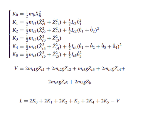
Here :

• K0 is the kinetic energy of one wheel
• Ki is the kinetic energy of ‘ith’ link of a single 4-bar linkage
• K is the total kinetic energy of on each side(left and right) of the bot
• V is the total potential energy
• L is the Lagrangian

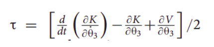
Where 𝞃 is the torque of the hip joint.

Methodology

Self-balance Mode

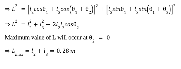
Calculating the length of the robot(L):

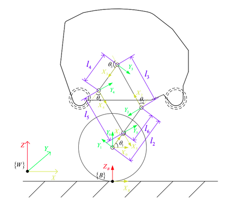
From the kinematics schematic of the robot, the following transformation matrices can be found out:

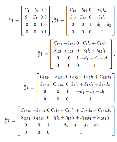
As coordinate {3} represents the motor’s position and {0} represents the wheel position, so, the length of the robot can be found by using the [0T3] matrix. (Assuming that center of mass of the robot lies near motor) The fourth column in [0T3] represents the coordinates of {3} in {0}. So, using distance formula, L=sqrt(sum of squares of first and second value in last column of [0T3]).

Calculating the mass of the robot (M):

The Mass of body is calculated as follows:

Upper Half of body consists of -

• 2 T-Motors - 180 g 2=360 g
• Lipo 6s (As T Motors requires 6s Lipo) - 720 g
• Microcontroller (Arduino) - 25 g
• Microprocessor (Raspberry Pi) - 10 g
• Buck Converter - 11 g
• 2 40 A ESC -30 g 2=60 g
• Lower Half of body consists of 2 Motors + Wheel (Negligible) = 360 g
• Total Mass M = 1546 g
• Lower Body Mass mb = 360 g
• For safety factor, we will consider 2 times of the calculated mass Therefore M = 3 kg, mb = 0.72 kg

So the values are taken as follows:

• r=0.03m
• M=3 kg
• mb=0.72 kg
• Ib=MLL
• Iw=4.5125*0.0001
• It=0.0225
• b=0.75
• g=9.82ms-2
• D=0.3m

The following model is made for the self-balancing mode using LQR controller:

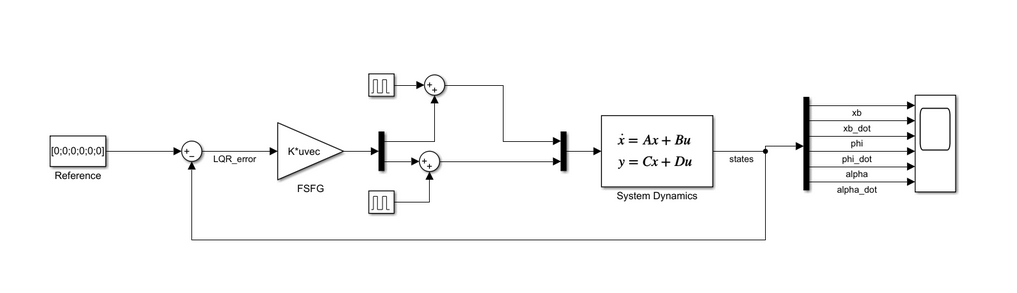
• Disturbance(using Pulse Generator) is added to the Plant input.
• The six states are observed in the o/p scope.

Jumping Mode

Trajectory Planning:

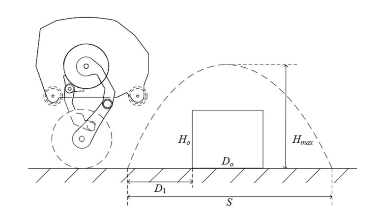
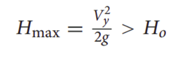
• We have taken Hmax as 0.5 m. This is used to estimate the vertical velocity of the robot when it is about to take off.
• S is taken as 0.2 m. This is used to estimate the horizontal velocity of the robot throughout the projectile.

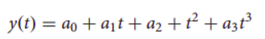
• We used this as the trajectory of the vertical component of the COM(hip joint) during the takeoff.

Control Block Diagram for Jumping Mode:

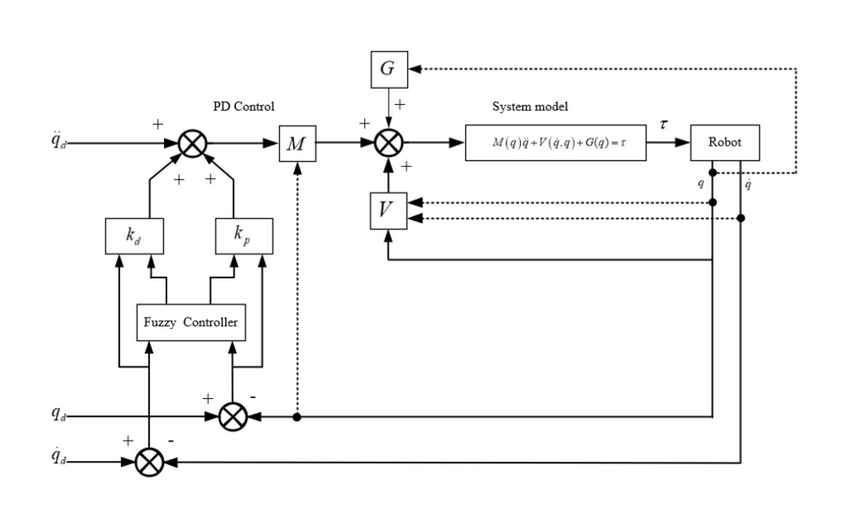
• This is the control block diagram which we used to control the hip joint angle and its derivative during the flight phase. qd, qd_dot and qd_ddot are the reference inputs. Where q represents the hip joint angle.
• Fuzzy rules are made to tune the delta_Kp and delta_Kd values which get added to constant Kp0 and Kd0 values to get PD gains.

Steps followed to establish this system:

• Obtained the Lagrangian from the KE and PE equations. This involves finding the transformation matrices of the COM of all the links wrt the world frame {W}.
• Next, we derived the equation of torque in terms of theta3, theta3_dot and theta3_ddot where theta3 is the hip joint angle.
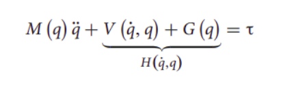
• We segregate the terms in the torque equation to find the following matrices:
  • Inertia matrix: M(q)
  • Coriolis force matric: V(q,q_dot)
  • Gravitational force matric: G(q)
• We used this information to build the following Simulink models:

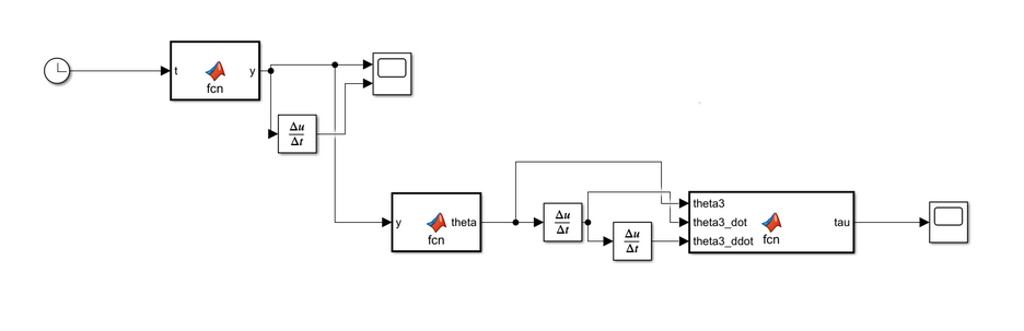
This estimates the torque as a function of time taking takeoff time as 0.45 seconds.

Control Design for q, q_dot control during takeoff:

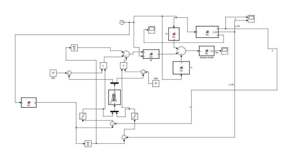
We built this system to control the q, q_dot while takeoff where q is the hip joint angle. But due to certain issues like the number of rules and membership functions of the fuzzy controller and due to the lack of proper reference trajectory equations, we could not get proper results for the torque and the control variables:

Results

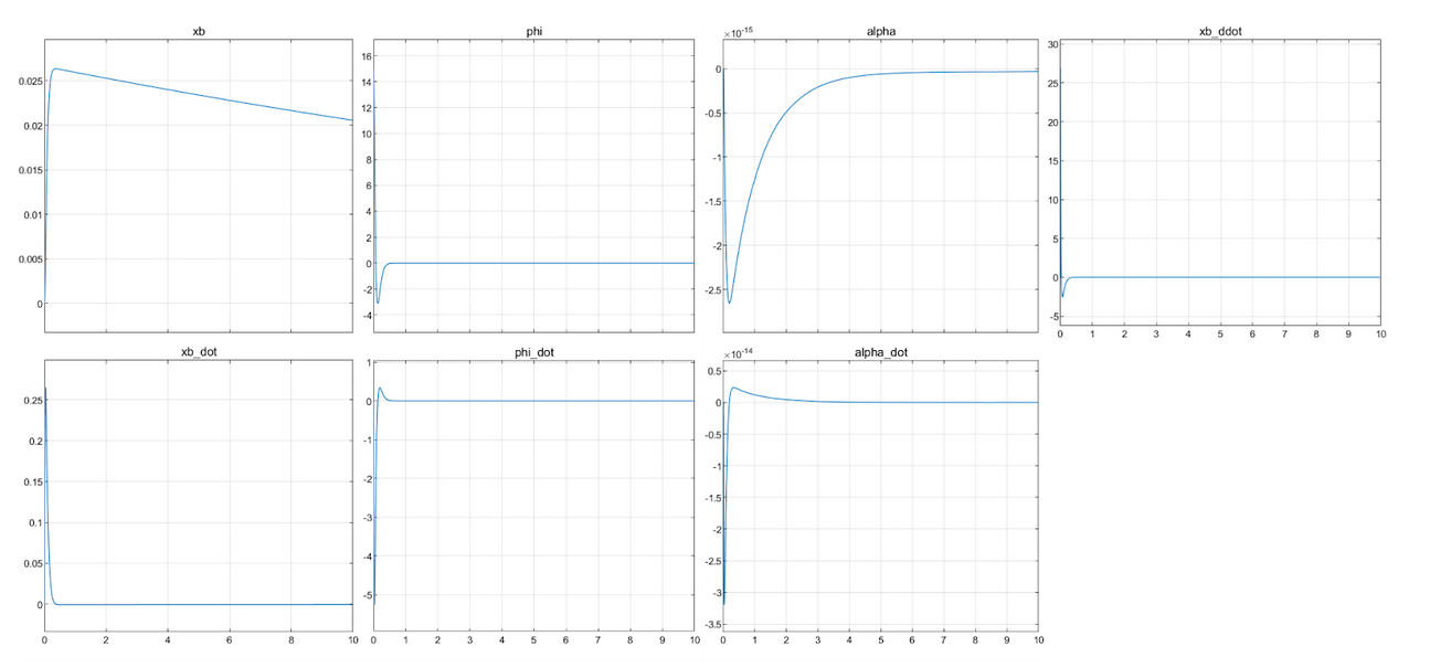
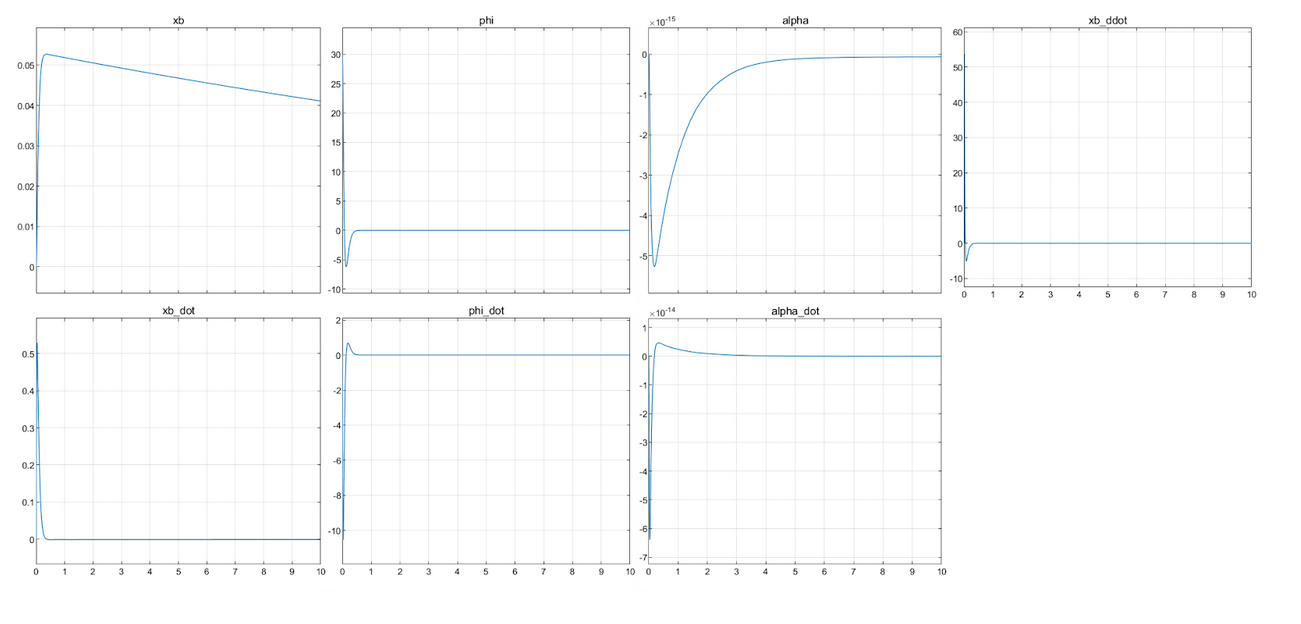
For testing, we set initial angles of robot as 15°, 30°, and 45°, and then we observed how it recovers by accelerating its bottom wheel

15°:

30°:

45°:

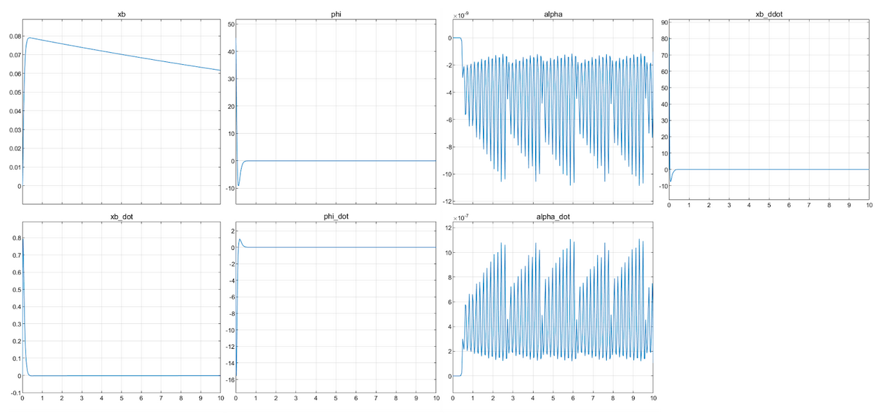
Using these results and aiming that the robot should be able to recover from 45° with max leg length, the specifications of motors for forward translational motion are found as:

• Max RPM = 254.77 RPM
• Max Torque = 9 N-m

Self balance Mode

Initial Angle=45 degrees, Hip angle=120 degrees

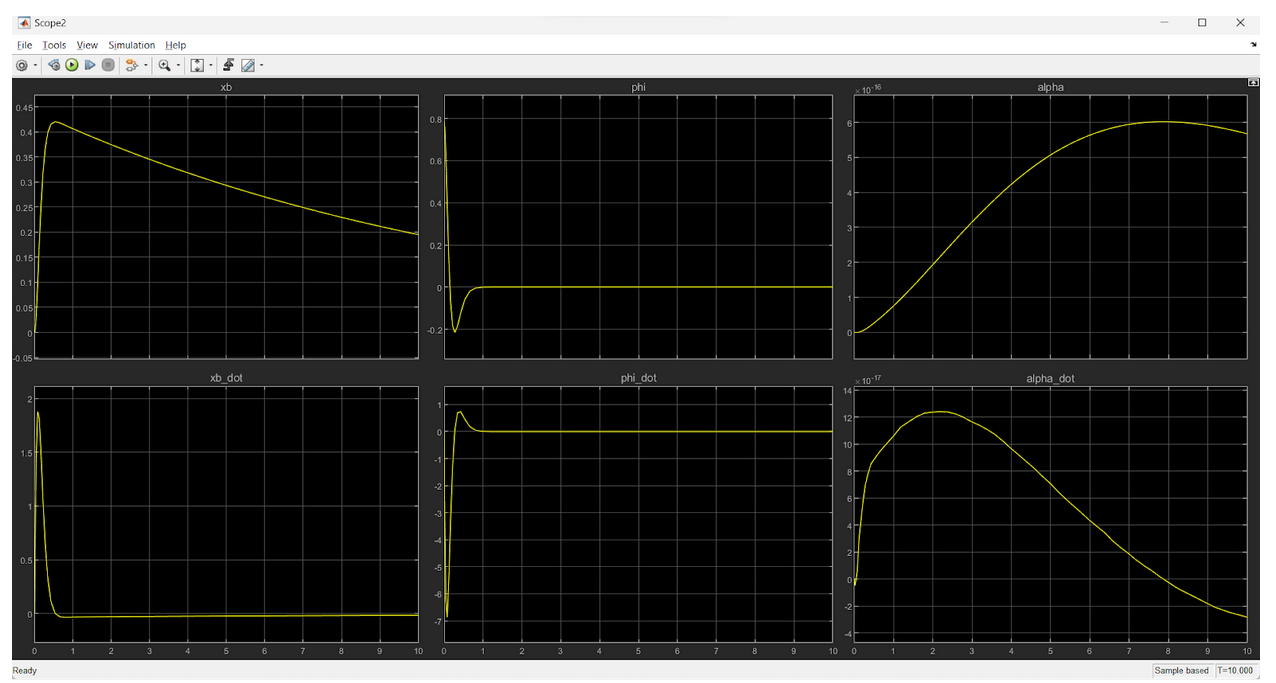
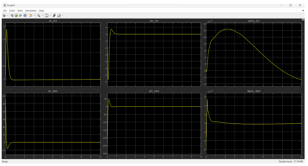
Initial Angle=60 degrees, Hip angle=120 degrees

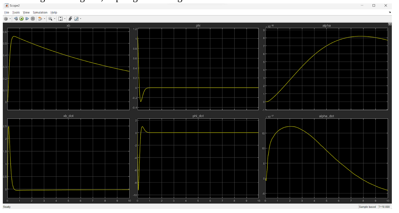
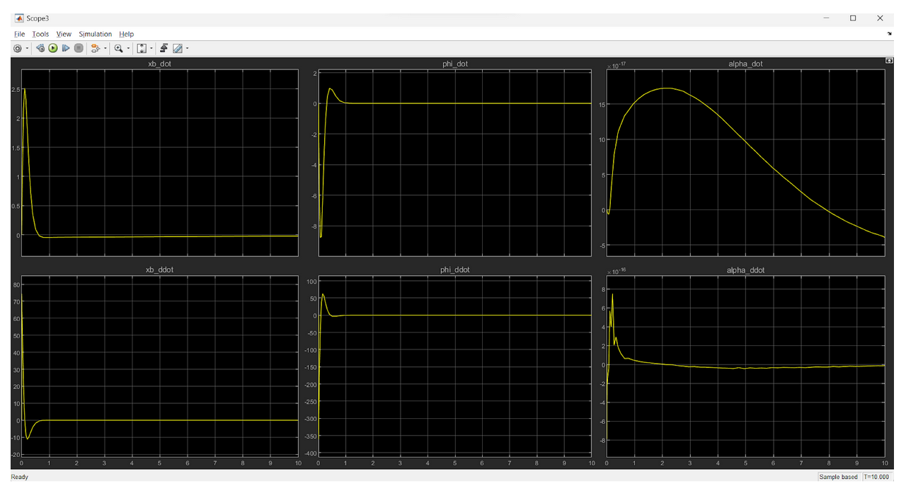
The simulation results can be used to obtain the motor specifications.

Jumping Mode

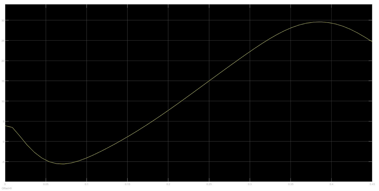
This is the variation of the torque. We can clearly see that the torque increases in the negative direction while retraction and then increases in the positive while jumping. (Note that the jumping phase involves retraction followed by jumping).

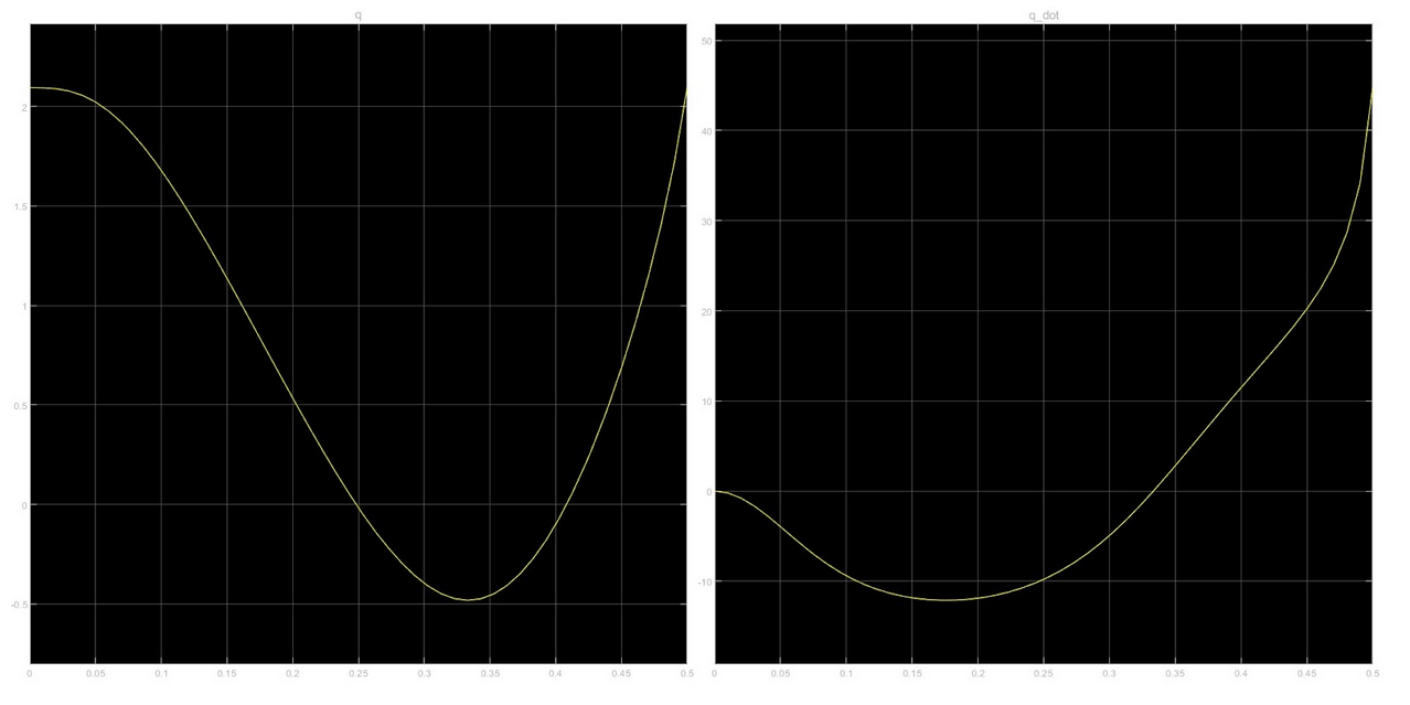
These are the plots for the q and q_dot. The parabolic projectile reference is taken into consideration.

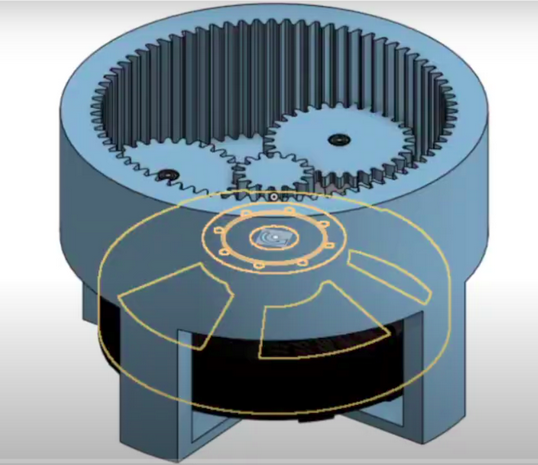
CAD

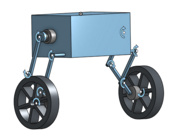
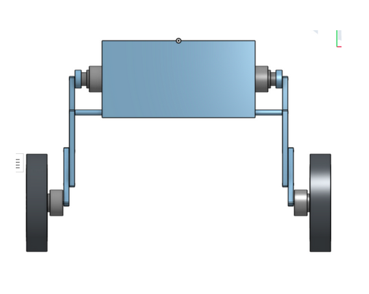
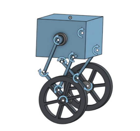
The CAD model for the robot is as follows:

Gearbox

The following work has been referred for this project: Link

Conclusion

• This work includes mathematical modeling of the wheeled biped and its implementation using LQR and Fuzzy PD controllers.
• MATLAB and Simulink results of the same have been presented.
• CAD design for the robot prototype and gearbox are also displayed.
• Future work includes:
  • Obtaining proper values of moment of inertias, and masses of various links to obtain the desired control and minimize the error of trajectory while considering the physical constraints.
  • The fabrication and testing of the physical system of the robot would be our target for the future.